- Background
- Shuffle bottlenecks
- Spark Magnet: Push-based Shuffle
- Other Solutions: Pull-based Shuffle
- References
Recently, our data infrastructure team deployed a new version of Spark, called Spark Magnet. It is said to offer 30% to 50% improvement in performance, compared to the original Spark 3.0.
Spark Magnet is a patch to Spark 3 that improves shuffle efficiency:
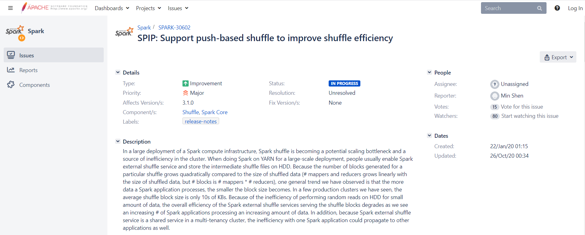
Provided by LinkedIn’s data infrastructure team, it makes use of the Magnet shuffle service, which is a novel shuffle mechanism built on top of Spark’s native shuffle service. It improves shuffle efficiency by addressing several major bottlenecks with reasonable trade-offs.
Background
Magnet is about shuffling, shuffling is the heart of MapReduce, which is the heart of distributed computing.
MapReduce
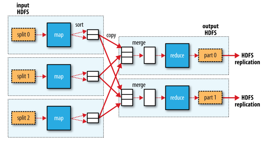
A MapReduce job consists of map tasks and reduce tasks. The computation is based on key-value pairs.
The input data is divided into splits. There would be one map task created for each split. Each map task is assigned a split as input.
After the map tasks are finished, their output are sorted by key. E.g., if the MapReduce job implements a group by operation, the key would be the group by key; if it is a join operation, the key would be the join key. Then, the sorted output is divided into partitions. There would be one partition for each reduce task.
Next, reduce tasks fetch their input data from the map tasks.
Lastly, the output of reduce tasks are written to HDFS (with replication).
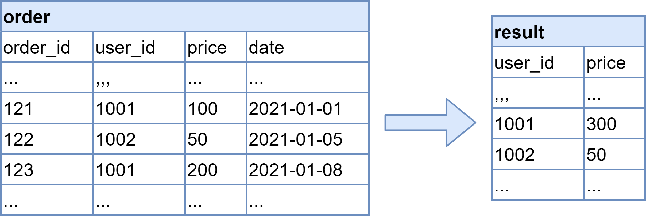
For example, suppose we want to compute the total amount of money each user spends on orders.
SELECT user_id, SUM(price) AS price FROM order GROUP BY user_id
This is how MapReduce implements the join operation:
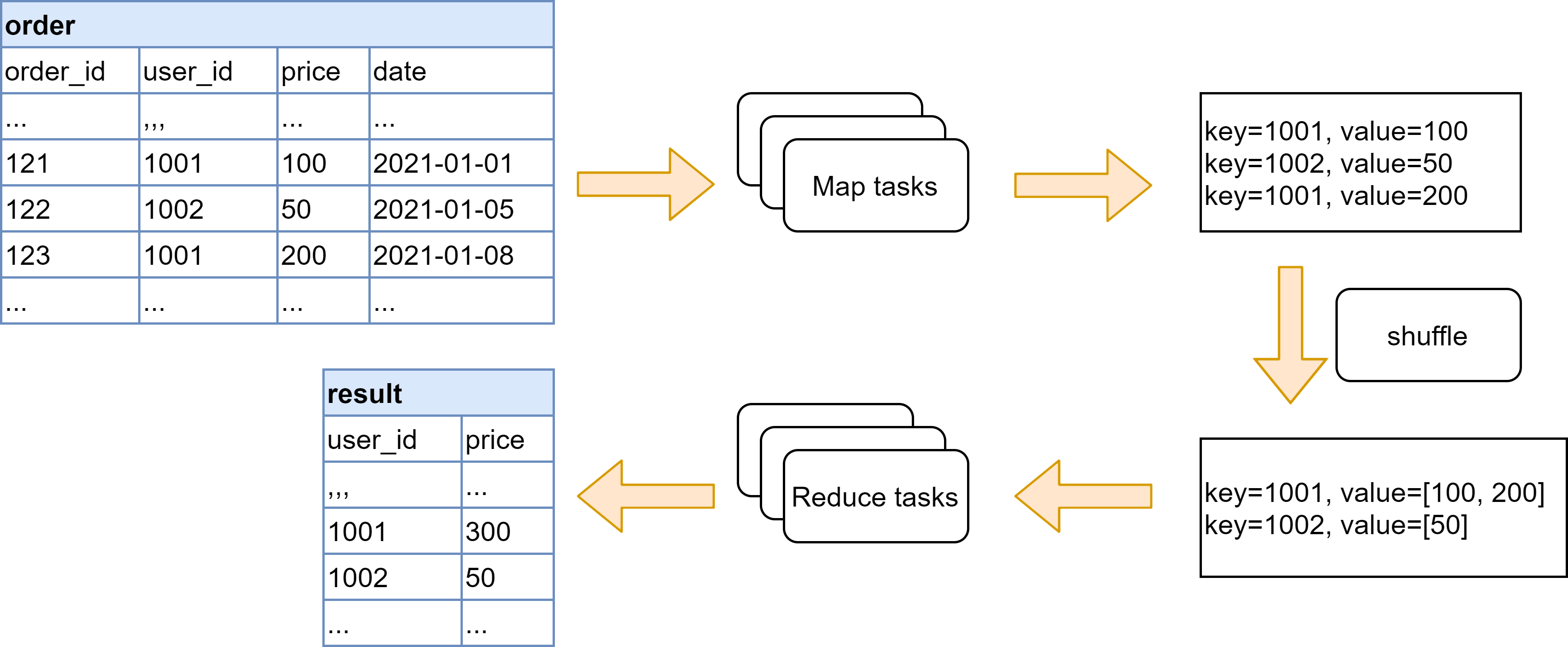
First, the map tasks extract the relevant key value pairs from the input data, i.e., the group by key, user_id, and value, price of the order. Then, the map output is sorted and aggregated by key. Finally, the reduce tasks sum the values for each key to produce the final output.
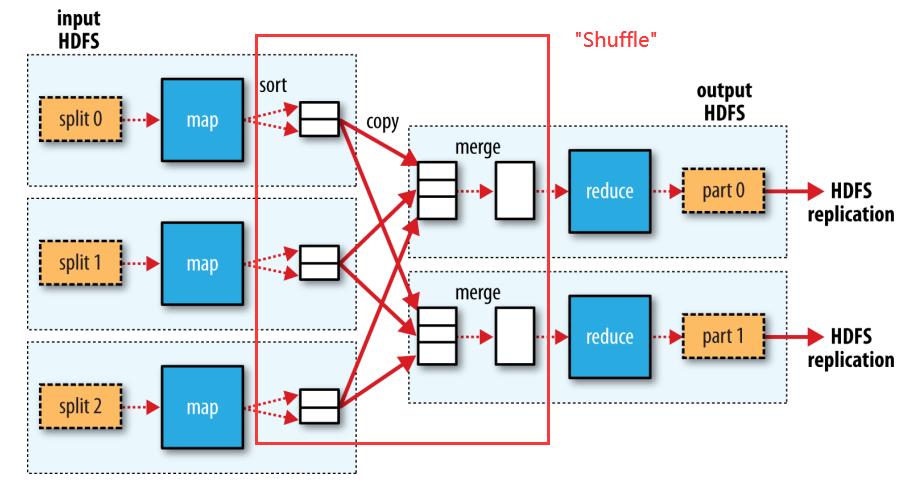
The process where the map tasks’ output are sorted and transferred to the reduce tasks is “the shuffle”. This is an all-to-all connection - each reduce task fetches its input from all map tasks. In the picture, there are 3 map tasks and 2 reduce tasks, so in total there are 3 * 2 = 6 shuffle connections.
Shuffle
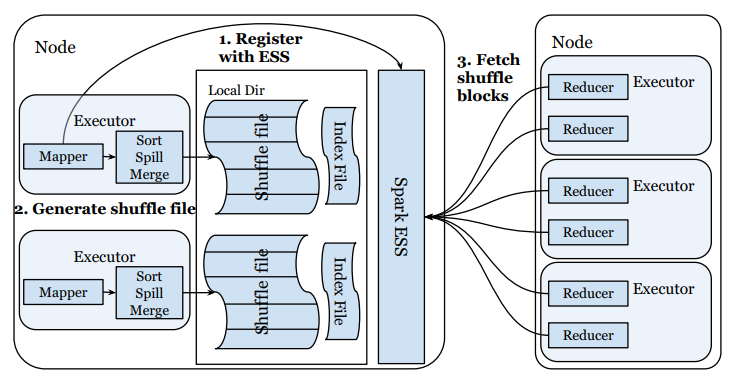
Now we zoom into the Shuffle operation. The picture shows two nodes in the cluster. On one node there are two executor processes, each running a map task. On the other node there are three executor processes, each running two reduce tasks.
Firstly, each executor registers with a Spark’s shuffle service instance located on the same node. This is for the shuffle service to know the location of the map task output, so that it can give this information to the reduce tasks later.
Secondly, shuffle files are generated from the map tasks’ output. After the map tasks are finished, their output is sorted in memory. If they can’t fit in memory, they will be spilled to disk. If there are several spills, they will be merged into a single file (hence the “sort, spill, merge”). Then the sorted output is divided into partitions based on the key, so that all records with the same key would be in the same partition. The partitioned shuffle files will be written to the node’s local disk.
Lastly, each reduce task connect with all the Spark shuffle service instances to fetch their input data (from the output of all map tasks).
Shuffle bottlenecks
There are several major bottlenecks when performing shuffle in a large cluster, including but not limited to:
- Inefficient disk I/O
- Unreliable shuffle connections
- Lack of reducer data locality
Inefficient disk I/O
Facts
- As input data size increases, the number of shuffle blocks increases quadratically while the shuffle block size decreases linearly.
- Suppose input data size is $D$. Suppose the amount of data a mapper or reducer can reasonably process is fixed, and based on this reasonable amount of data, we need $M$ mappers and $R$ reducers. Then as input data size increases, we would have more and more shuffle blocks that are getting smaller and smaller.
- Spark’s shuffle service reads only one shuffle block for each fetch.
- Individual shuffle blocks are accessed in random order.
| Input data size | Number of mappers | Number of reducers | Number of shuffle blocks | Shuffle block size |
|---|---|---|---|---|
| $D$ | $M$ | $R$ | $M*R$ | $\frac{D}{M*R}$ |
| $2D$ | $2M$ | $2R$ | $4(M*R)$ | $\frac{D}{2(M*R)}$ |
| $10D$ | $10M$ | $10R$ | $100(M*R)$ | $\frac{D}{10(M*R)}$ |
As a result
So in a large cluster, there will be a lot of small random reads during shuffle fetch stage. This is slow on hard disk drives, because the disk pointer need to perform a lot of seeks operations, and (unlike writing operations) it can’t make use of caching. (prevalent storage solution as SSDs are expensive).
Moreoever, existing solutions are not ideal:
- We can tune Spark configurations to create shuffle blocks with more reasonable size, but this is difficult, especially when the input data and logic change frequently.
- Automatic-tuning can also be done, but there are trade-offs that make it difficult to obtain improvement in overall performance.
So this is something that cannot be solved by tuning configurations and calls for infrastructure-level optimizations.
Unreliable shuffle connections
Facts
- All-to-all shuffle connections: Each reduce task’s input data is from all map tasks’ output, so each reduce task needs to connect with all shuffle service instances to get their input data.
- Theoretically, there would be $M * R$ connections.
- In reality, reducers on the same executor share one outgoing connection, and mappers registered with the same Spark shuffle service instance share one incoming connection. So the total number of shuffle connections is the number of executors times the number of shuffle service instances.
- Connection issues are common in large clusters.
- If a shuffle connection fails, Spark would fail the entire shuffle fetch stage, this would trigger expensive retries to re-generate the shuffle data that can’t be fetched.
As a result
There are frequent shuffle fetch failures with expensive retries.
Lack of reducer data locality
Facts
- Data locality is Hadoop’s feature to put data and compute tasks on the same node, so that data access is fast without needing expensive and unreliable network links.
- Reducers enjoy little or no data locality because they need to fetch input data from all mappers.
As a result
Shuffle fetches can be slow and unreliable in large clusters.
Spark Magnet: Push-based Shuffle
Spark Magnet is based on a concept called push-based shuffle.
 |
 |
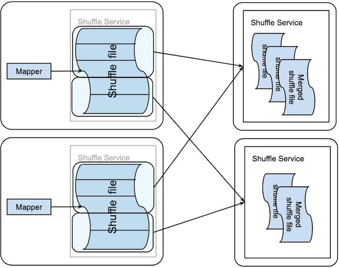
First, map tasks push their output to the remote Magnet shuffle service.
- Best-effort basis
- Note that the Magnet shuffle service is remote, unlike the Spark shuffle service instance which locates on the same node. However, this loss of locality is made up by the performance boost enabled by the following steps.
- The remote push is decoupled from the map tasks, so push failures do not lead to map task failures.
- There is a configurable size limit to this push, so shuffle blocks larger than this limit are not pushed. This avoids pushing skewed blocks.
Then, the Magnet shuffle service merges the shuffle blocks it receives into one file per shuffle partition.
- Best-effort basis: Not all blocks are merged. The picture shows both merged files and the original, unmerged files.
- This step converts small random reads during shuffle fetch to large, sequential reads.
- This step introduces double writing of the shuffle blocks, since the shuffle data needs to be written once before merging, and once after merging. But this drawback is still better than small random reads because writing, unlike reading, can benefit from caching (the pointer just needs to find the next empty slot). Moreover, the double writing effectively saves a second copy of the shuffle data, which improves reliability.
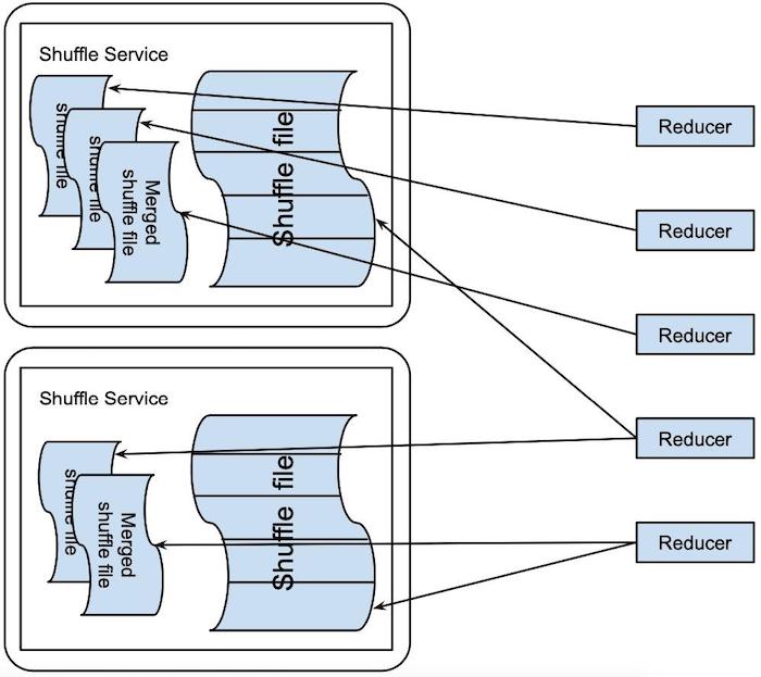
Lastly, reducers fetch input data from the shuffle service.
- Best-effort bassis: They first try to fetch from the merged shuffle files, and if it fails, they fall back to fetching the original, unmerged files. This prevents triggering expensive retries to re-generate the shuffle data.
- Reducer data locality: Executors are launched based on location of shuffle services, where the majority of reducer input is merged.
To sum up:
| Bottlenecks | Spark | Magnet | Magnet’s complications |
|---|---|---|---|
| Disk I/O | Small random reads. | Large sequential reads of merged shuffle files. | Double write, but can benefit from caching. |
| Shuffle connection | Low fault tolerance, expensive retries. | Fault tolerance by replicating shuffle blocks in merged shuffle files. | New risk of failure in push/merge, but won’t trigger expensive retries. |
| Reducer data locality | Little or none. | Launch executors based on location of shuffle services, where majority of reducer input is merged. |
Other Solutions: Pull-based Shuffle
There is another family of shuffle service optimization efforts based on the idea of “pull-based shuffle”. Instead of mappers pushing shuffle blocks to the shuffle service, the shuffle service pulls blocks from mappers. Authors of Spark Magnet argue that Magnet has several advantages over pull-based shuffle because of this distinction.
References
- Spark Magnet JIRA ticket: https://issues.apache.org/jira/browse/SPARK-30602
- Spark + AI Summit 2020 talk on Spark Magnet: https://databricks.com/session_na20/tackling-scaling-challenges-of-apache-spark-at-linkedin
- LinkedIn’s engineering blog post on Spark Magnet: https://engineering.linkedin.com/blog/2020/introducing-magnet
- Spark Magnet paper: http://www.vldb.org/pvldb/vol13/p3382-shen.pdf
- Pull-based shuffle paper: https://dl.acm.org/doi/10.1145/3190508.3190534
- Hadoop: The Definitive Guide: https://www.oreilly.com/library/view/hadoop-the-definitive/9780596521974/