Background
Given a stream of events:

How to process it?
Batch Processing
We can process the stream in batches. In this example, each batch contains a day’s worth of data.
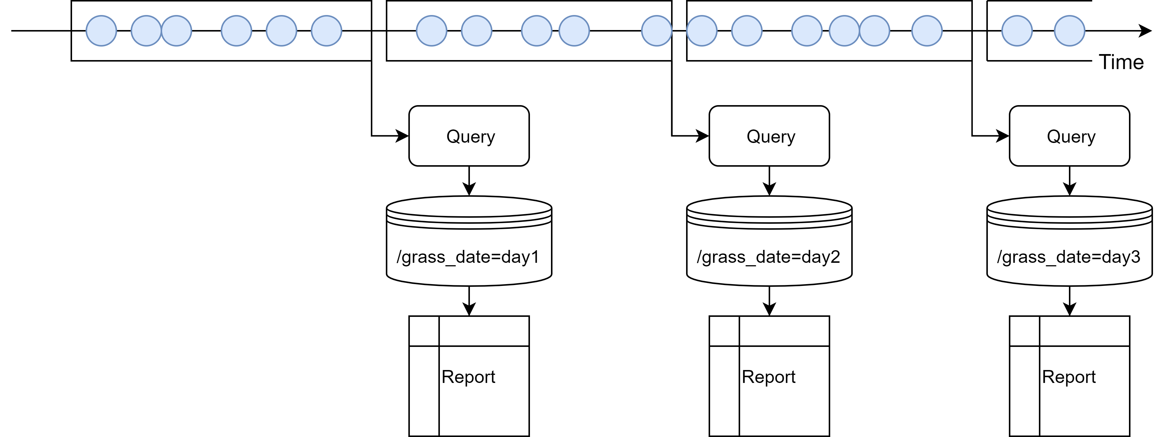
Note that there is a delay: Data of day n is only ready for processing on day n+1.
Stream Processing
On the other hand, we can also use stream processing, which processes the stream continuously.
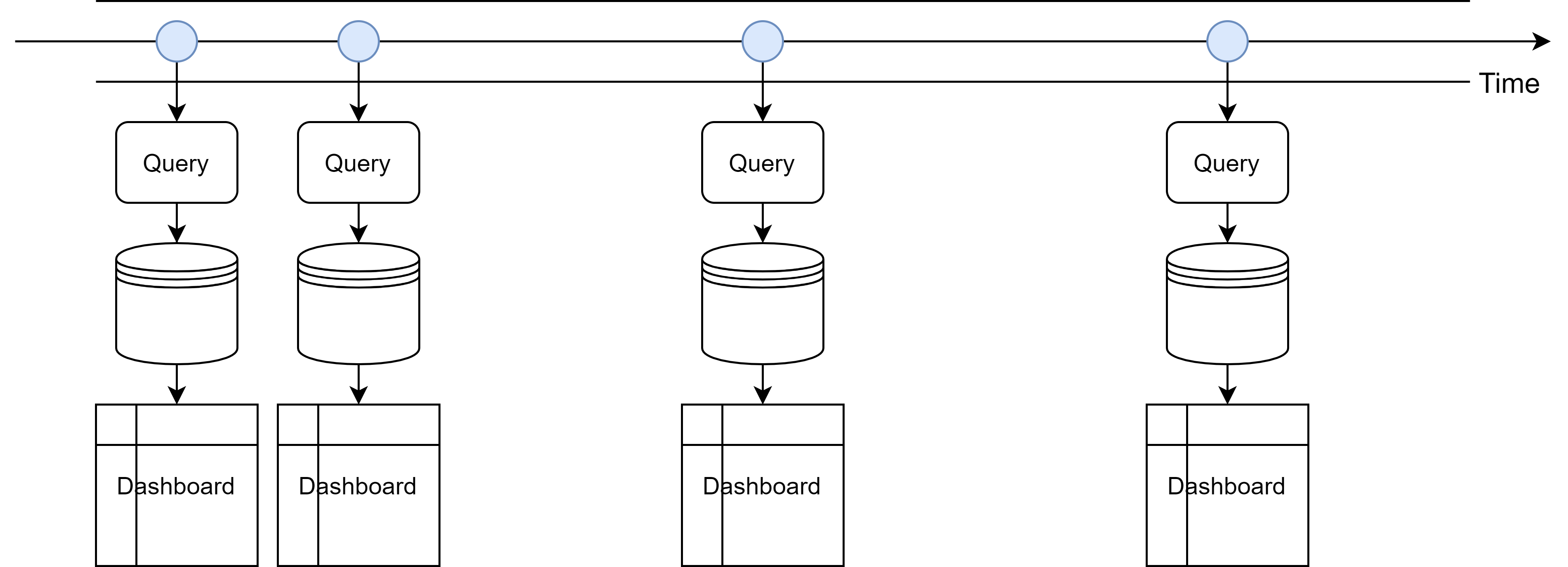
This allows producing real-time results since events are processed as they come without the need for batch accumulation.
Concepts
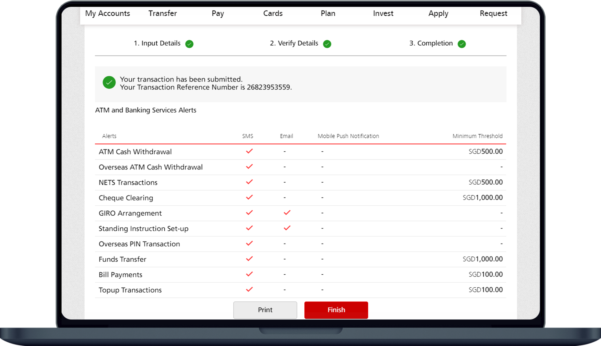
Suppose we want to design fraud detection logic for bank transactions.
A straightforward approach would be:
Approach 1: Send alert of amount > threshold
We can set a threshold, and send alert if the transaction amount exceeds the threshold.
Suppose we have the following transactions. We just need to go through each transaction one by one and see if it exceeds the threshold.
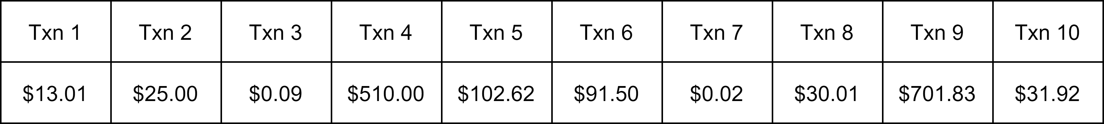
E.g., if the threshold is \$500, then txns 4 and 9 will trigger alerts.
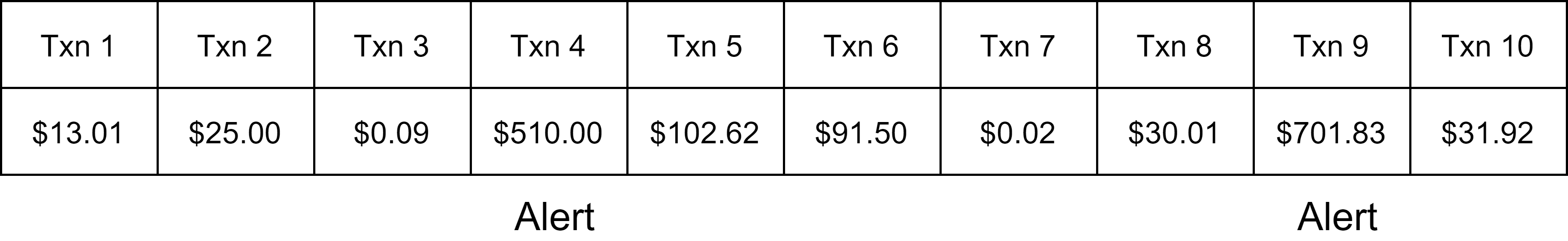
The operation of comparing each transaction with the threshold is an example of stateless operation, since it does not require remembering any information about previous events (“state”) as we go.
Stateless operation. Operation on event stream that looks at one event at a time, i.e., does not require remembering information (“state”) about previous events.
This first approach is very crude, as there could be a lot of false alerts. On the other hand, if we are able to remember information about previous events, can we improve the fraud detection logic?
State
Approach 2: Look for patterns - small amount transaction immediately followed by large amount
Turns out that criminals who steal credit cards would usually test the cards by making a small transaction first, and if the test works, they then begin transferring large amounts.
So we can set a maximum threshold for small transactions and a minimum threshold for large transactions, and look for small transaction immediately followed by large transaction.
E.g., if “small” transactions means < \$1 and “large” transactions means > \$500, then txns 3 and 4 would be detected as fraud.
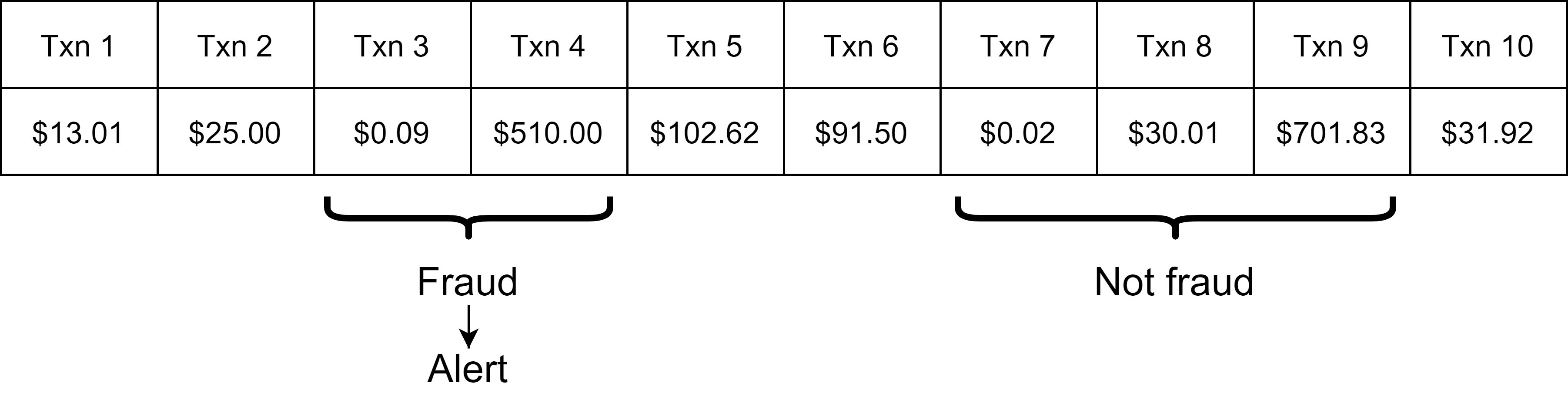
Note that txns 7 and 9 won’t be detected as fraud because there is a txn 8 in between that breaks the pattern.
The operatgion of first finding a small transaction and then looking for a large transaction that immediately follows it is an example of stateful operation, because we need t remember whether the last transaction was small or not.
Stateful operation. Operation on event stream that requires remembering information about previous events.
Can we do better still?
Let’s look at txns 3 and 4 closely. They fit the pattern of small transaction immediately followed by large transaction. But “immeidately” here only means there are no other transactions in between. Due to the lack of time dimension, we don’t know how close the transactions are temporally. On the other hand, it’s reasonable to assume that for a real fraud, the large transaction should be within a short time period of the small transaction. So if the transactions are, say, a few days apart, then it wouldn’t make sense to report them as fraud.
State + Time
We can improve this approach by adding a time condition:
Approach 3: Look for patterns - small amount transaction immediately followed by large amount within some time limit
We limit the pattern to some time period.
E.g., if the time limit is 1min, then txns 3 and 4 won’t be detected as fraud.
This is an example of timely operation, which is an extension of stateful operation in which time plays a role.
Timely operation. An extension of stateful operation in which time plays a role.
- E.g., aggregations based on time periods (“window”) - we will come back to this topic later after introducing more concepts about time.
Time
Consider:
Example. Compute the total number of requests the server receives every 5 min.
There is only one notion of time in this example, i.e., system time of the processing machine (in this case, the server) when each request is received.
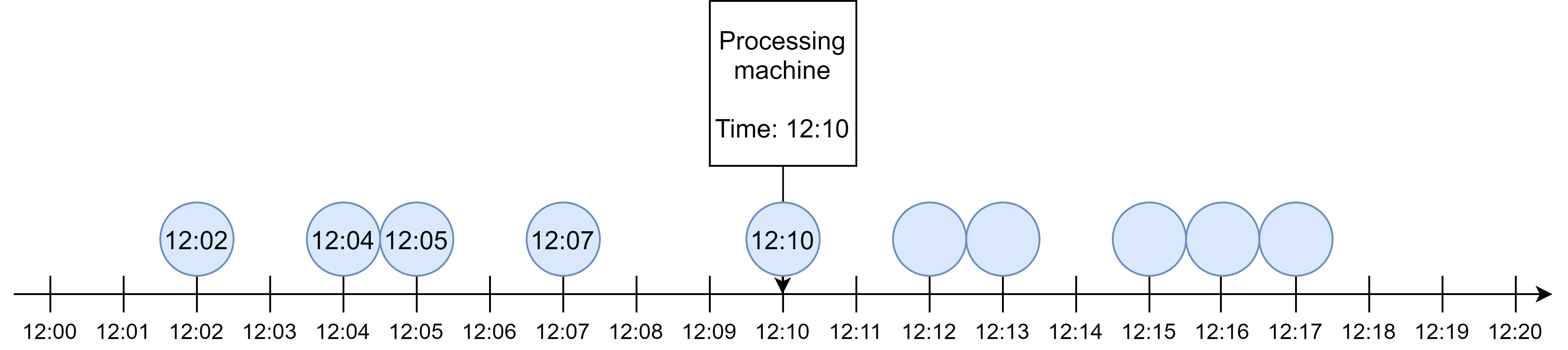
This notion of time is known as processing time.
Processing Time
Processing time. System time of the processing machine when each event is received.
-
Not deterministic
Results computed using processing time depend on the speed at which the events arrive at the processing machine. This may change if the events are replayed.
-
Low latency
Don’t need to wait when aggregating by processing time periods, since all events within the period of say 12:05 to 12:10 would have all arrived by 12:10 by the definition of processing time. (This is not true for the other notion of time we introduce next.)
To introduce the other notion of time, consider:
Example. Compute the total number of online orders made every 5 min.
There are two notions of time in this example:
- System time of the processing machine when the order record is received - this is the processing time we discussed before.
- System time of the buyer’s device when the order is made - this is known as event time.
Event Time
Event time. System time of the producing machine when each event was produced.
-
Deterministic
Event time is embedded in the events before they arrive at the processing machine. This won’t change even if the events are replayed.
-
Latency:
Events don’t always arrive in the same order in which they are produced. There may be delays, and as a result, events may arrive out-of-order, i.e., events produced earlier may arrive later than events produced later. So if we want to aggregate by event time periods, we may need to wait for out-of-order events.
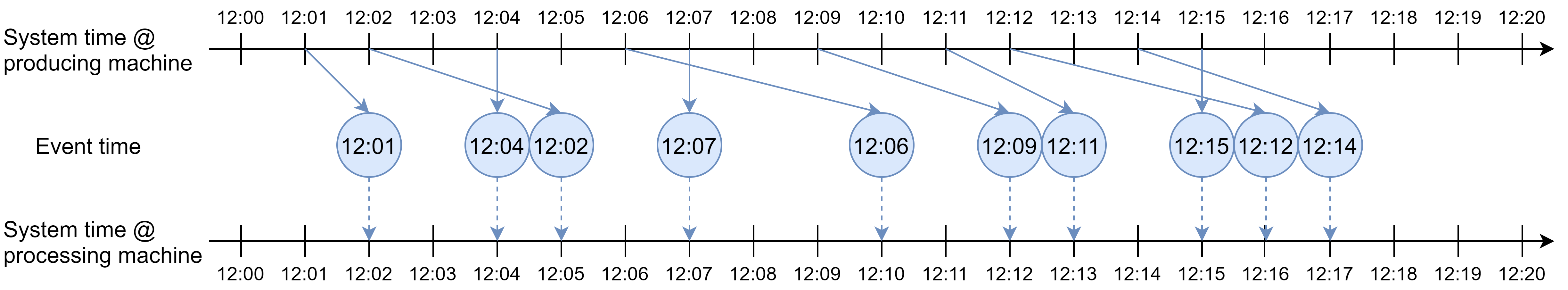
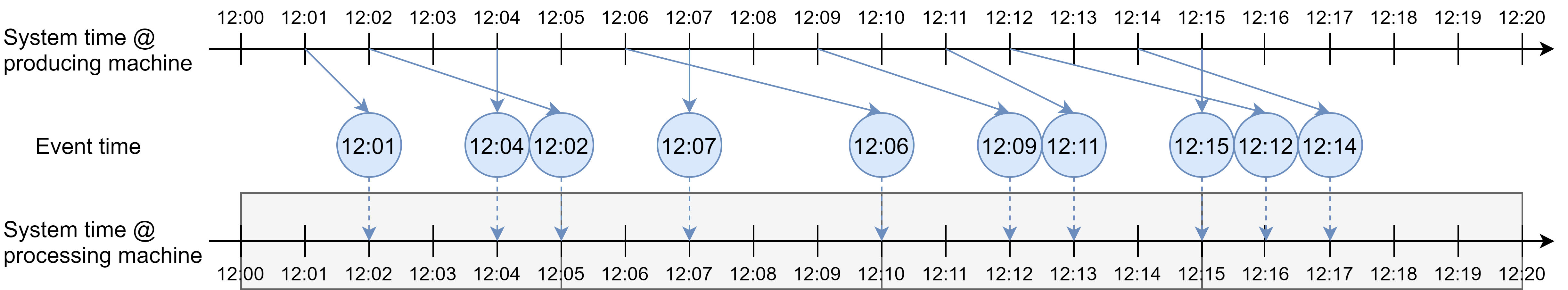
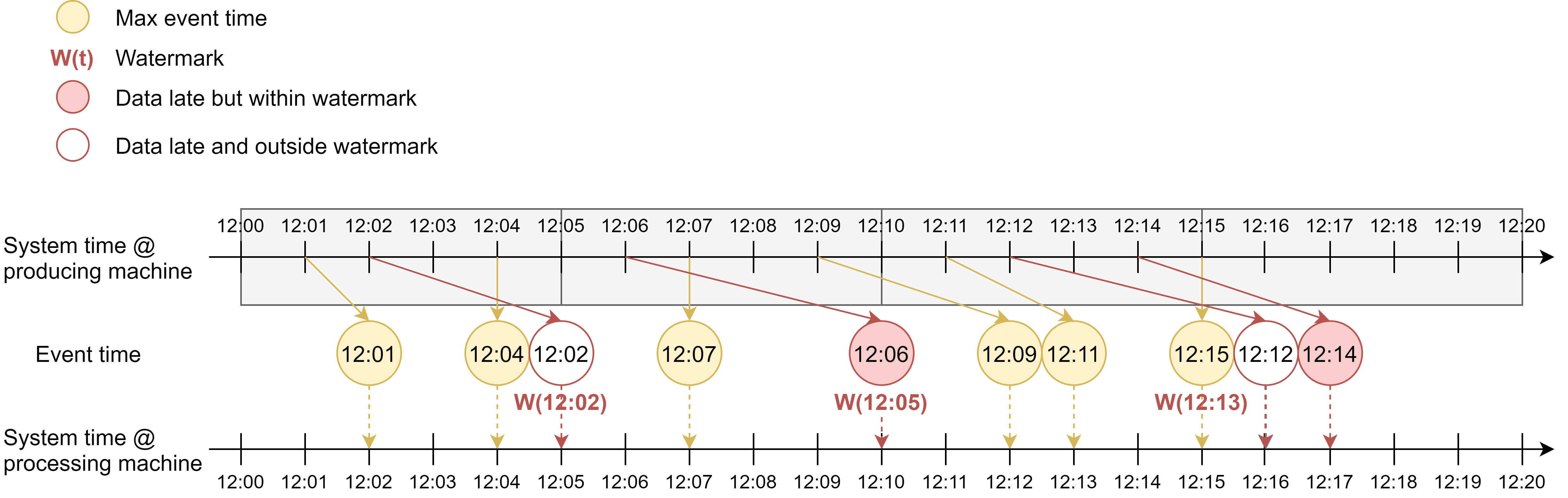
Consider these orders created at the producing machine (in this case, buyer’s device) at 12:01, 12:02, 12:04, etc.

During transit, the events become scrambled. E.g., the order created at 12:02 is delayed and is now behind the order created at 12:04.
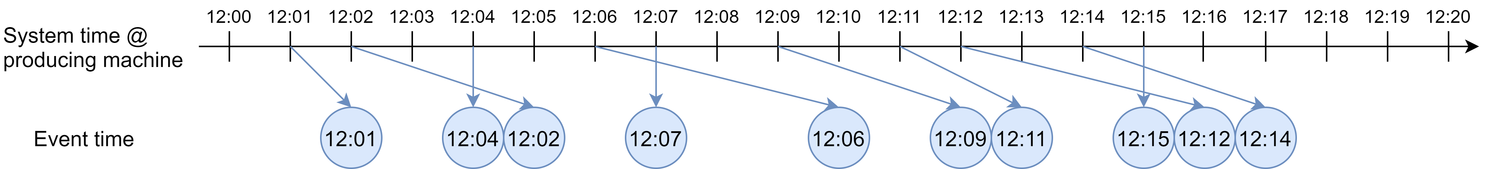
As a result, when the orders arrive at the processing machine, they arrive out-of-order. Except for the orders created at 12:04, 12:07 and 12:15, all the other orders are delayed. Some orders are delayed by so much that they arrive later than orders created later.
Processing Time vs. Event Time
To sum up, event time is the time when each event occurred, and processing time is the time when each event is observed by the processing pipeline.
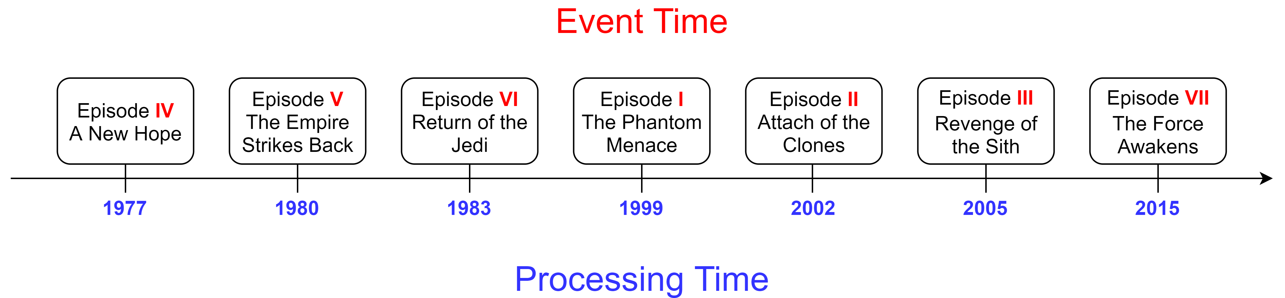
We can use Star Wars to better understand the two notions of time. Here’s a timeline of the 7 star wars movies. The blue timeline below is when each movie was released, i.e., processing time. The red timeline above is when the events in each movie actually occurred in the storyline, i.e., event time. We see that the movies are not made in the order in which they took place in the storyline.
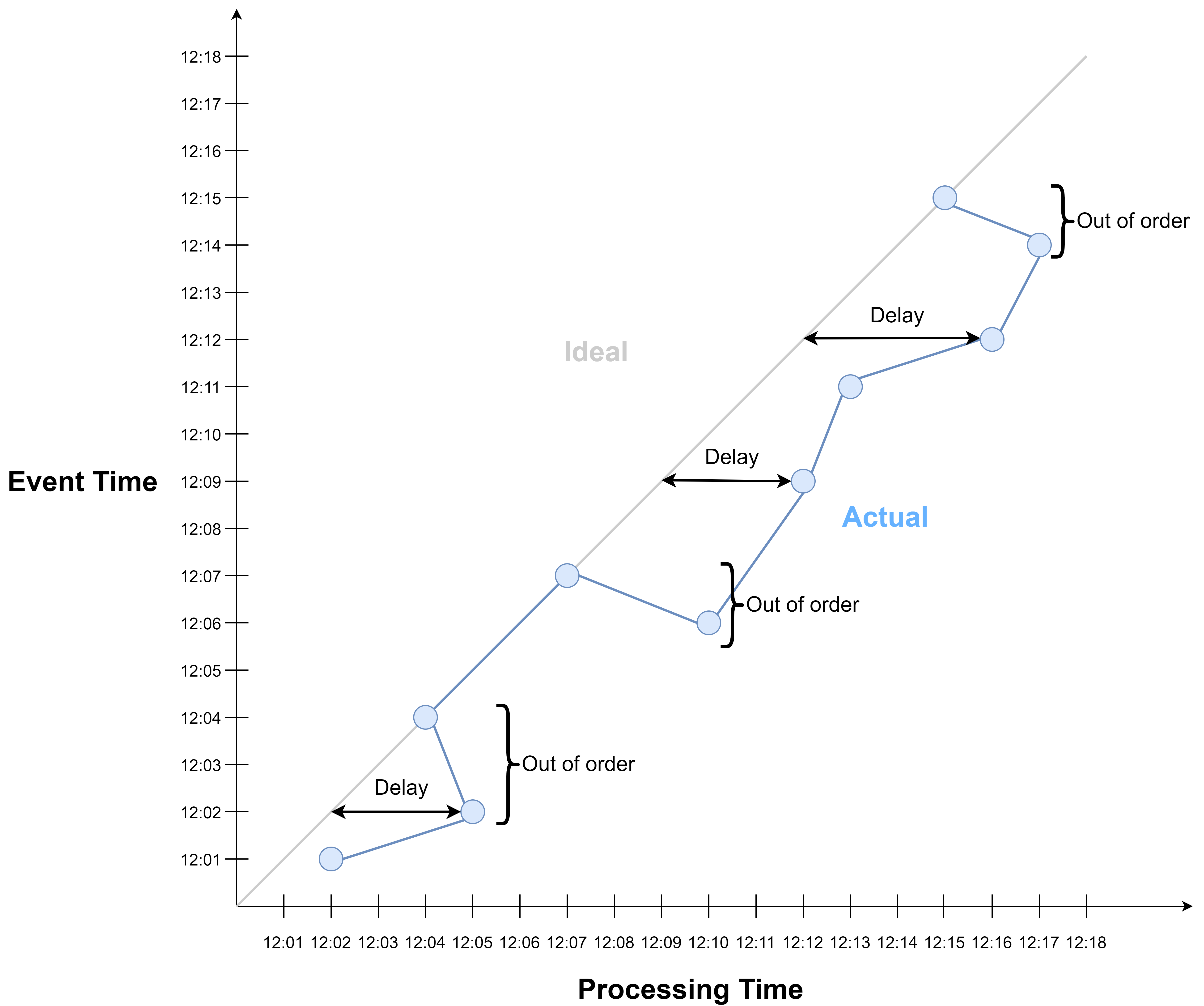
The difference between processing time and event time is captured by a concept called event time skew. This is the deviation of processing time progression from event time progression.
In the ideal world, processing time exactly corresponds to event time:
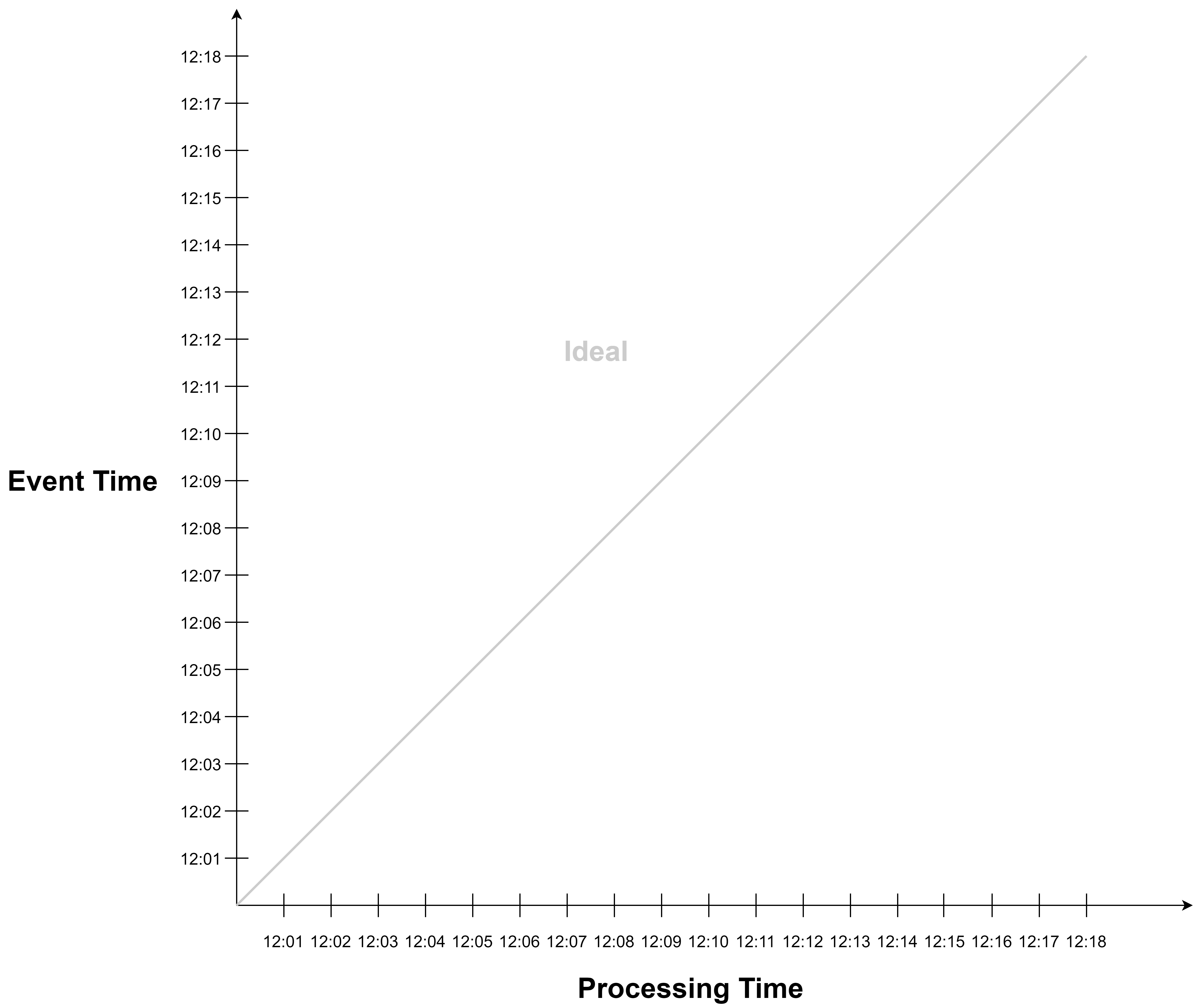
In reality, processing time deviates from event time due to event delay.
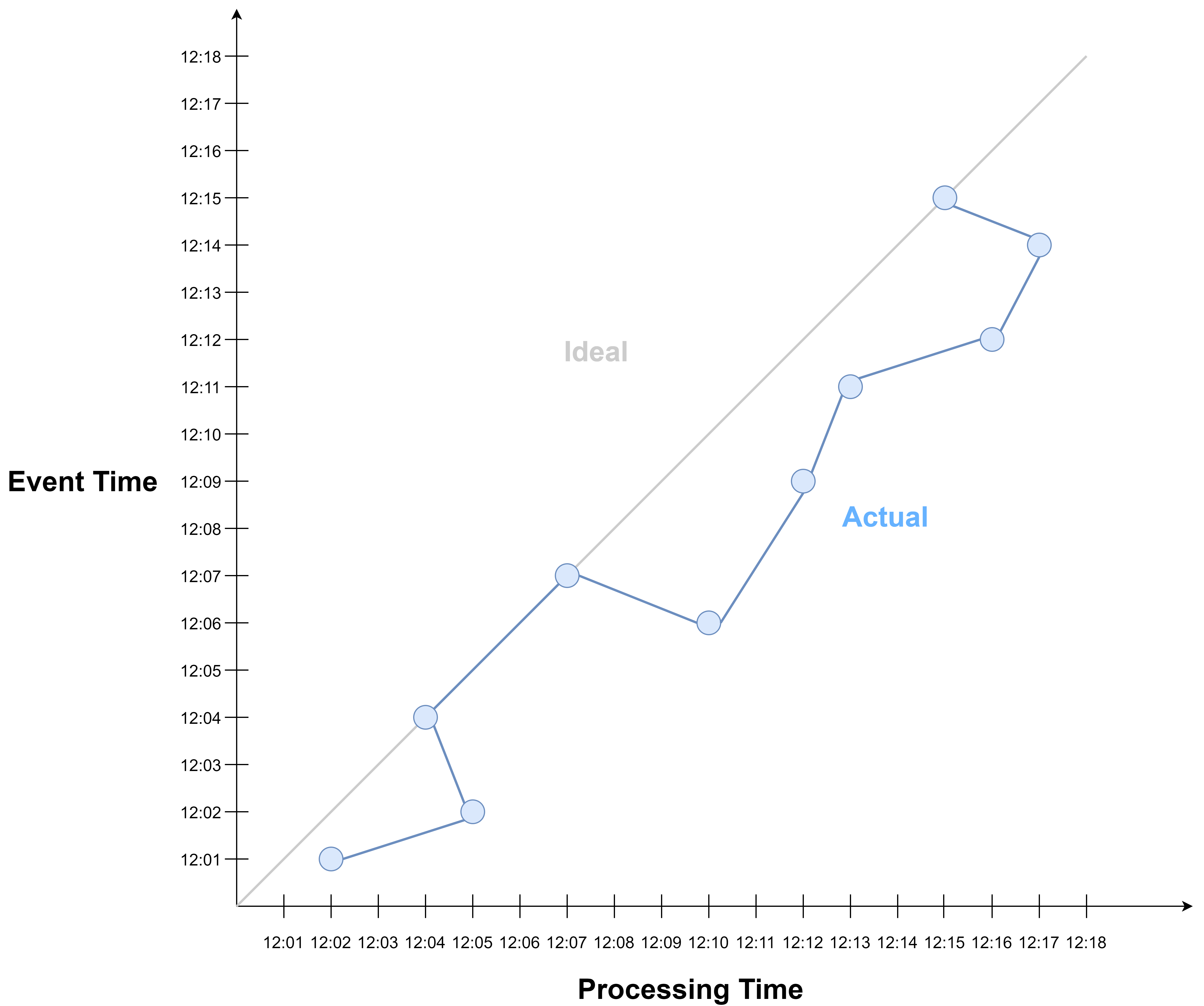
These delays may cause events to be out of order with respect to event time.
Having gone through the notions of time, we can now proceed to explore their applications. An important application is time-based windowing.
Windowing
In stream processing, we often need to perform aggregations by key and time periods (“window”). E.g.,:
- Number of ad clicks per ad per minute
- key: ad, window: 1 min
- Sum of electricity usage per household per hour
- key: household, window: 1 hour
- Maximum temperature per sensor per minute
- key: sensor, window: 1 min
These are all examples of windowing.
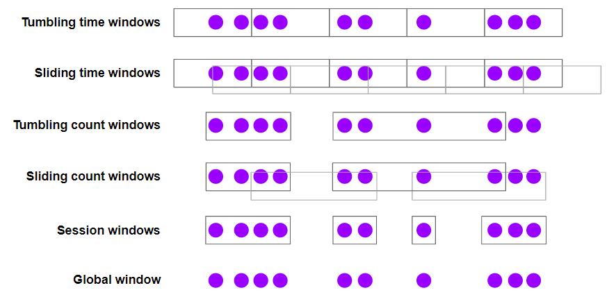
Windowing. Mechanism to slice up a data stream into bounded chunks for processing.
- Time-based windows: Tumbling window, sliding window, session window
- Count-based windows: Tumbling count window, sliding count window
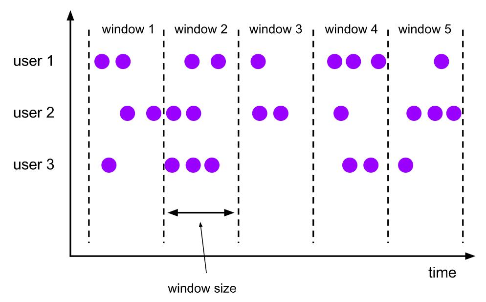
Let’s revisit this example:
Example. Compute the total number of online orders made every 5 min.
This is a use case of tumbling time window.
Whether we should use processing time or event time depends on the use case. Here we can interpret the example to mean event time because it refers to the time when the orders are made. But even if the use case requires event time, we can choose to use processing time or event time depending on our priorities.
Processing Time Window
If we use processing time, we are trading accuracy for low latency.
We get low latency because we don’t need to wait for late events.
But we lose some accuracy in view of event time, because each processing time window may:
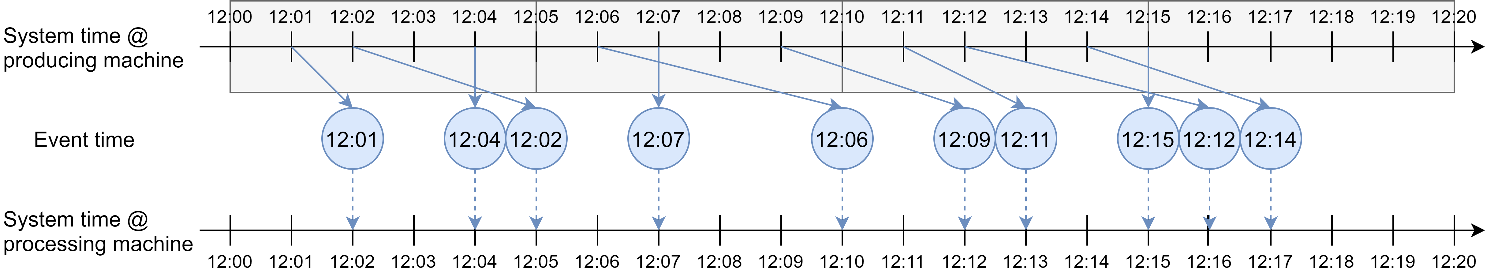
- contain events that belong to the previous (event time) windows but fall into the current processing time window due to delay.
- miss out events that belong to the current (event time) window but are delayed such that they fall into the next processing time windows.
E.g., the processing time window from 12:10 to 12:15 contain the event occurred at 12:09 which belong to the previous window, and miss out events occurred at 12:12, 12:14 which fall into the next window.
Here is another view of the situation:
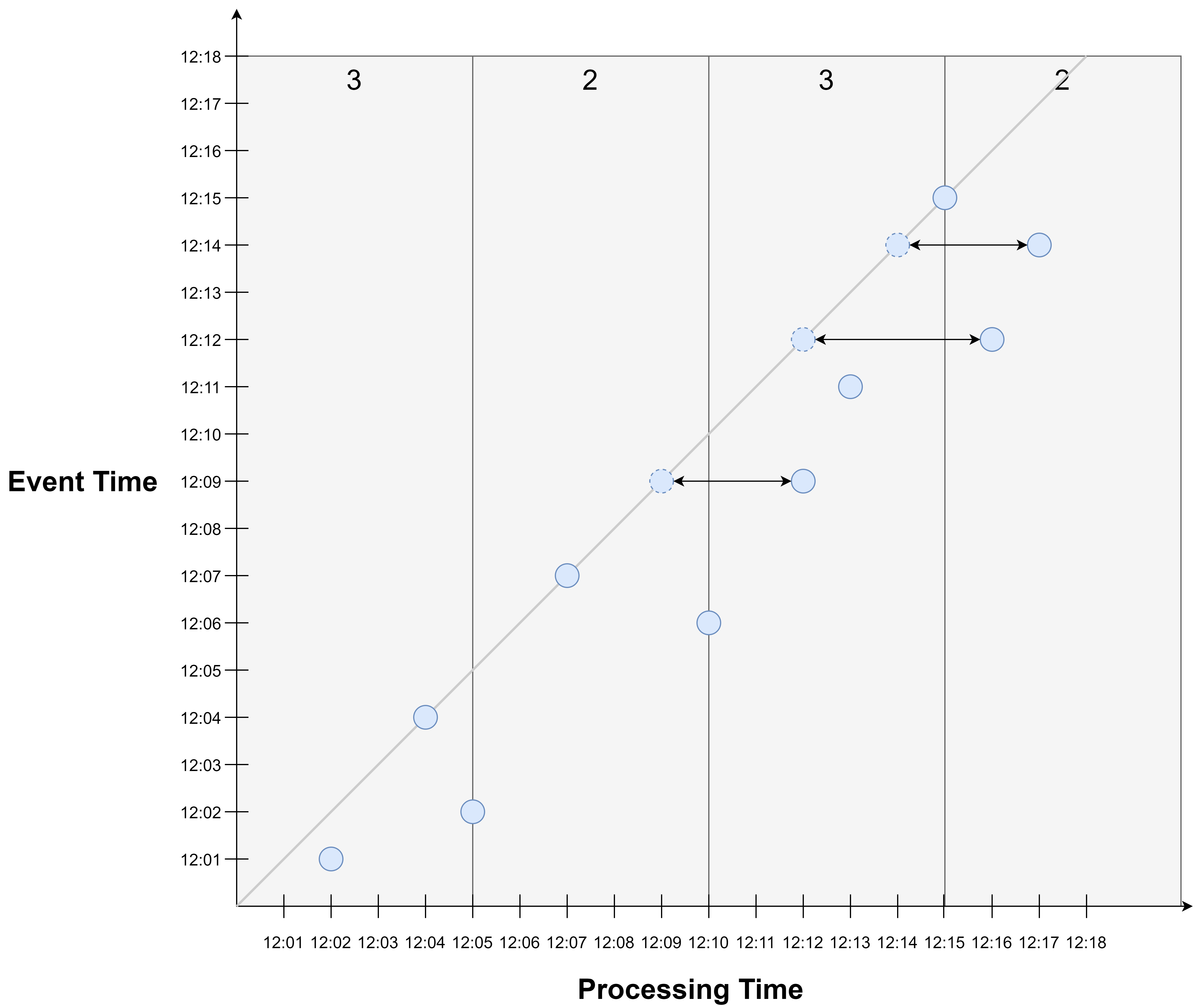
Due to event time skew, events may fall into later processing time windows than they would in event time. E.g., the events occurred at 12:09, 12:12, and 12:14 all fall into a later window than they would have had they arrived on time.
This is a source of inaccuracy when using processing time window to approximate event time windows: The processing time window of a given time period does not accurately contain the events occurred during that period in event time.
That said, using processing time window to approximate event time window is a valid option if:
- we value timely results and are ok if the results may be inaccurate for individual windows (with the assurance that eventually all events would be accounted for), or
- we don’t have event time available.
Event Time Window
If we have available event time data and are ok with waiting for late events, then we may choose to use event time window for aggregation.
In this case, we are trading latency for accuracy: When aggregating for the window 12:05-12:10, we need to wait for the event that occurred at 12:09. Same for the window 12:10-12:15, where we need to wait for the events occurred at 12:12 and 12:14.
This begs the question: How long should we wait?
Here are some observations:
- In order to do better than processing time window, we need to wait for some time.
- But we can’t wait forever - at some point we need to stop waiting, make the assumption that no more late events will arrive, and move forward.
- We can imagine there exist different waiting policies
This is where watermarks come in.
Watermark
Watermark. A watermark of time $t$ ($W(t)$) declares that event time has reached time $t$, i.e., we expect no more events to arrive with a timestamp $t’ <= t$.
The way we generate watermark determines our policy to wait for delayed events. The watermarks help us keep track of event time progression., which gives us a measure by which we can decide to stop waiting for late events.
Here are some examples of the different policies to generate watermarks:
| Based on | Strategy | Assumption |
|---|---|---|
| Processing Time | Watermark = Processing time - fixed delay Generated periodically (in processing time). |
Event arrival delay <= fixed delay |
| Event time | Watermark = Max event time - fixed delay Generated periodically (in processing time). |
Event arrival delay <= fixed delay |
| Event time | Watermark = Max event time - fixed delay Generated each time event time advances. |
Event arrival delay <= fixed delay |
| Event | Watermark = Event.watermark | Events carry watermark information |
| … | … | … |
The first policy assumes that watermarks are delayed by a fixed amount on top of processing time. It generates watermarks periodically in processing time.
The second and third policies assume that watermarks are delayed by a fixed amount on top of the maximum event time observed so far. They generate watermarks periodically or when event time is advanced by the arrival of a new event with a new maximum event timestamp.
The first three policies assume that events delays are bounded by a fixed, maximum delay.
The fourth policy doesn’t manage the watermarks itself, but simply extracts them from events. This is for cases where the events carry watermarks themselves.
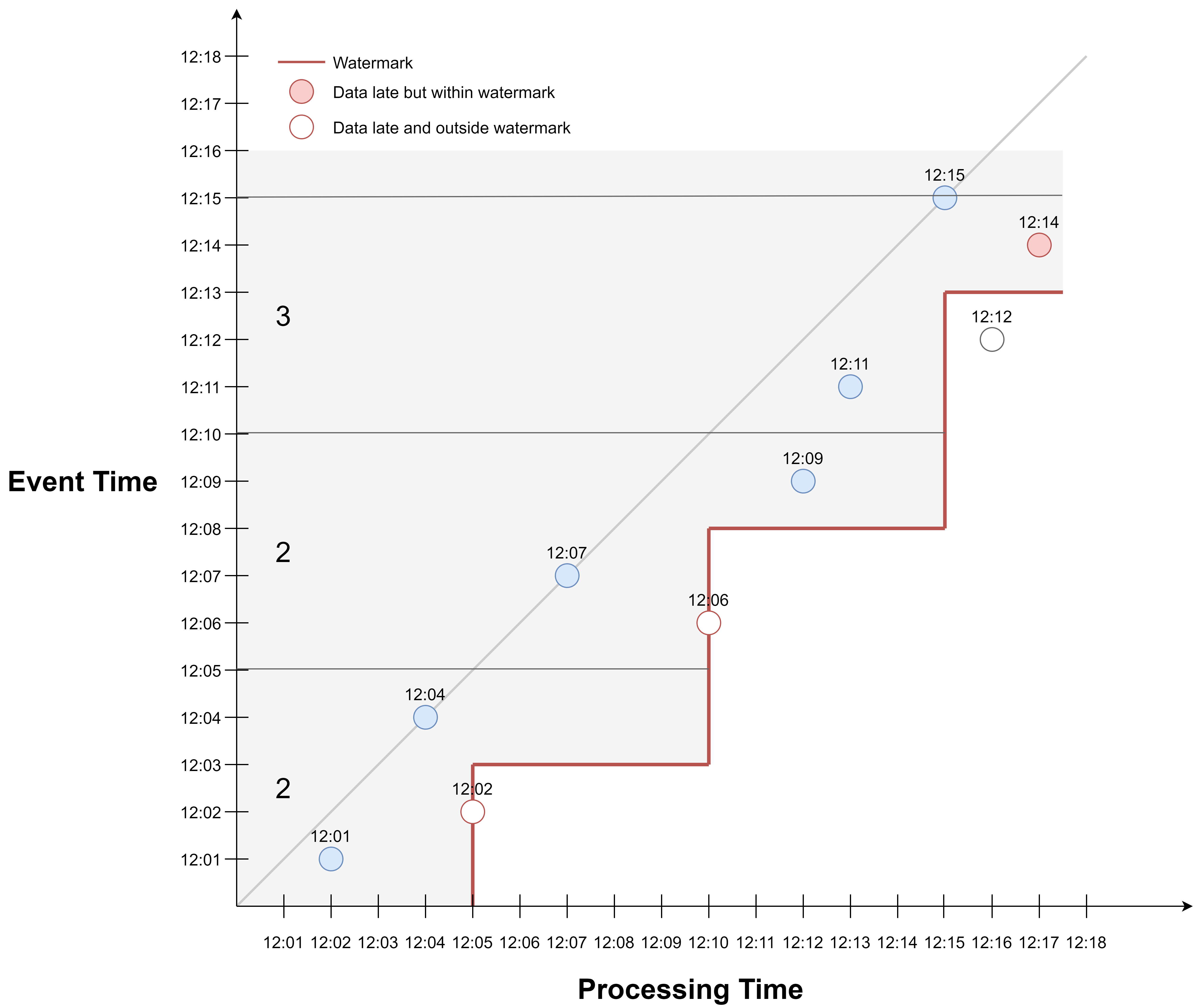
Here is an example of the first policy, where watermark is defined as processing time delayed by 2 min, generated every 5 min.
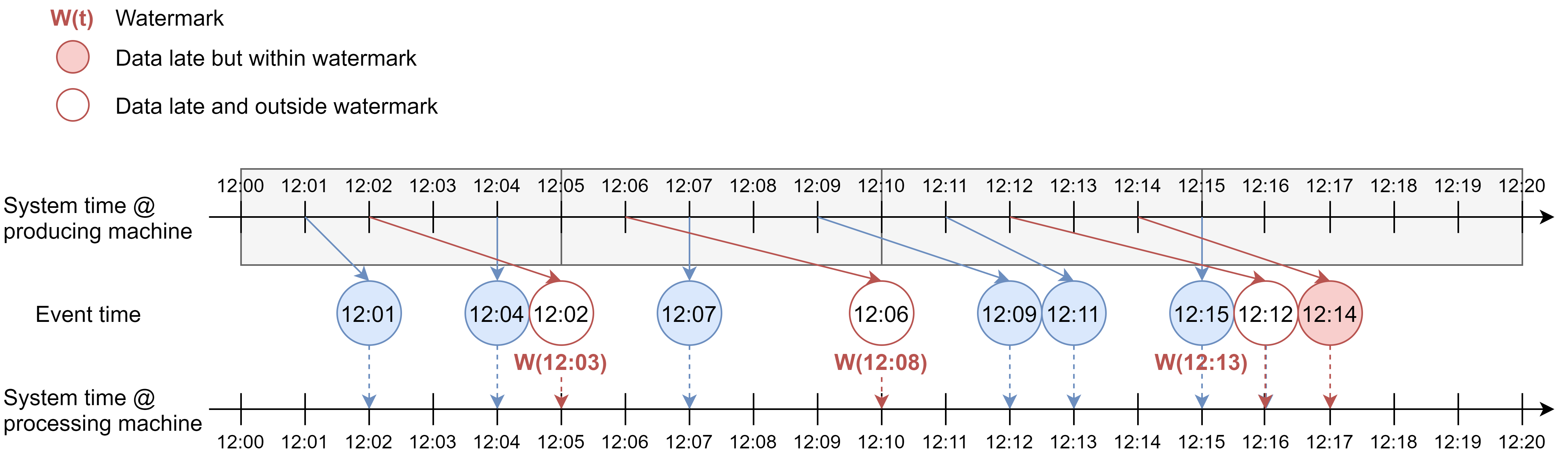
If we apply event time tumbling window of 5 min, the aggregation will be done in these event time windows based on when the event occurred, it’s just that events outside of the watermark are excluded from the aggregation. So our waiting policy is actually to wait for events that are late but inside watermarks (the red circles), and stop waiting for events that are outside watermark (the white circles). So we would get 2 events in the first window, 2 events in the second window, and 3 events for the third window.
Here is another view of the example. Events that are on or to the right of the red watermark line correspond to events that are outside the watermark and will be excluded from the aggregation.
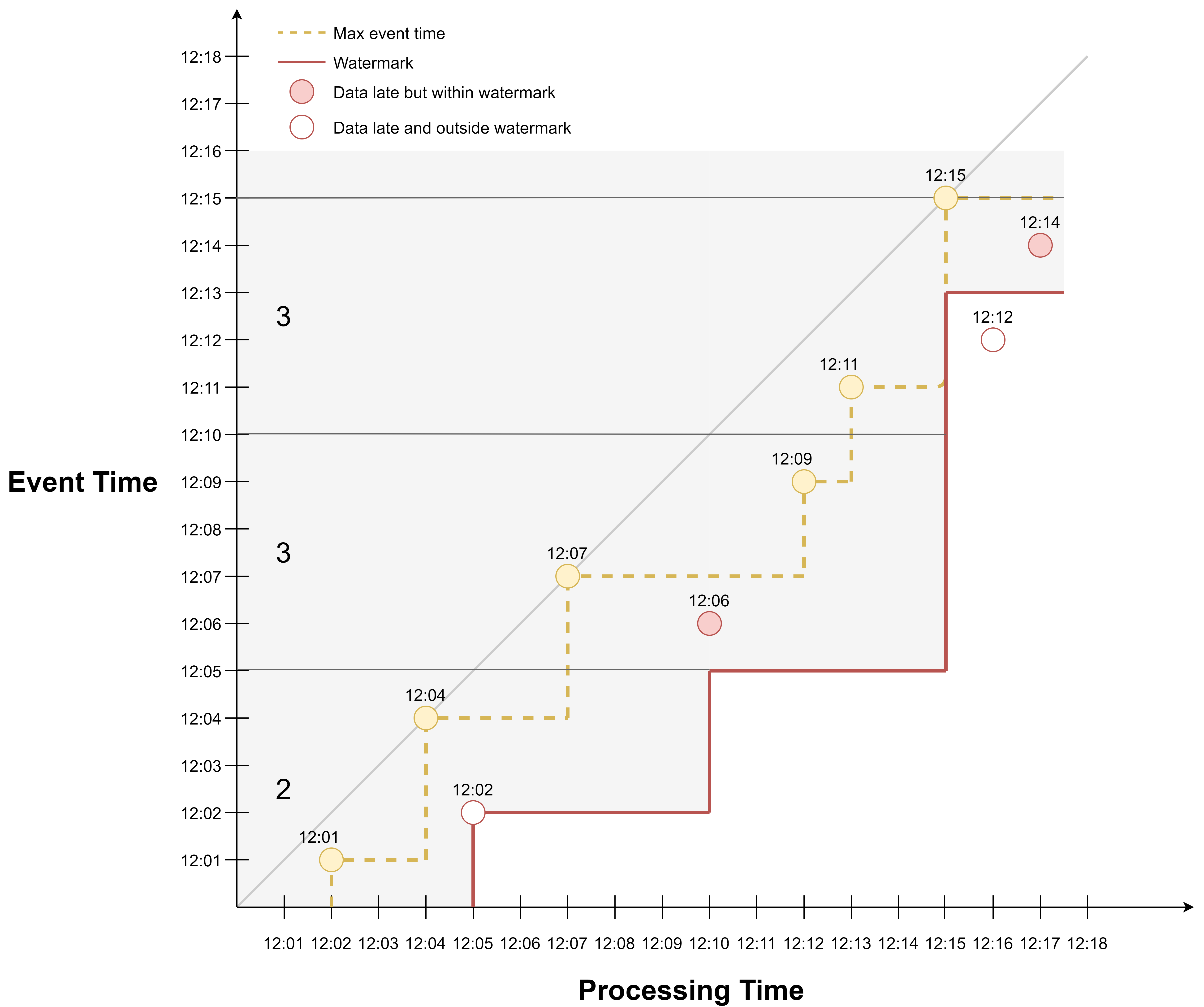
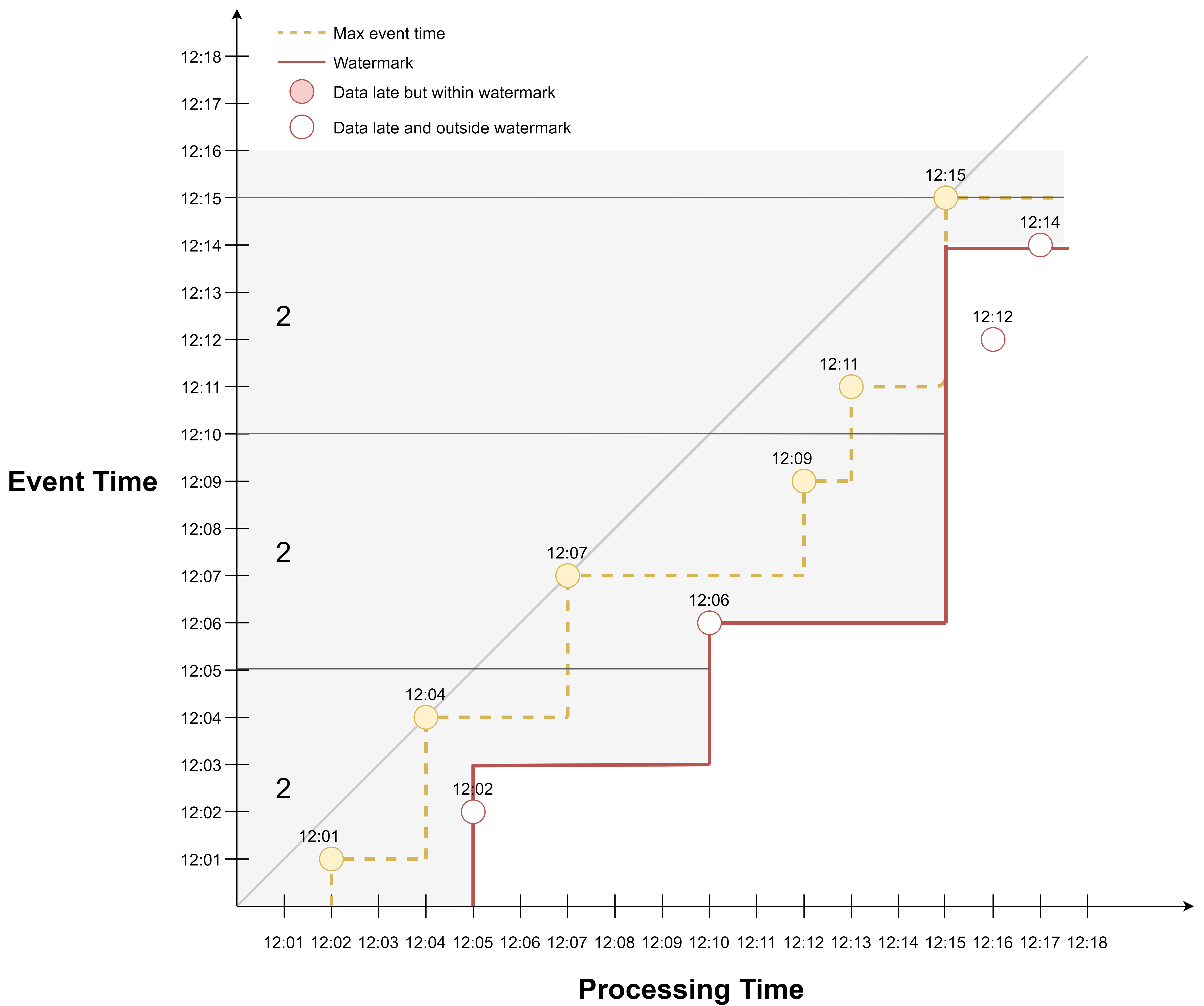
Here is an example of the second watermark generation policy, where watermark is defined as maximum event time observed so far delayed by 2 min, generated periodically.
The first watermark is generated at 12:05. The maximum event time so far is 12:04, so the watermark timestamp is 12:02. This says that from 12:05 onwards in processing time, we stop waiting for events that arrive with a timestamp <= 12:02. So the event occurred at 12:02 will be excluded.
The second watermark is generated at 12:10. The maximum event time so far is 12:07, so the watermark timestamp is 12:05.
The third watermark is generated at 12:15. The maximum event time so far is 12:15, so the watermark timestamp is 12:13. So the event occurred at 12:12 will be excluded.
If we apply event time windowing, we would get 2 events in the first window, 3 events in the second window, and 3 events for the third window.
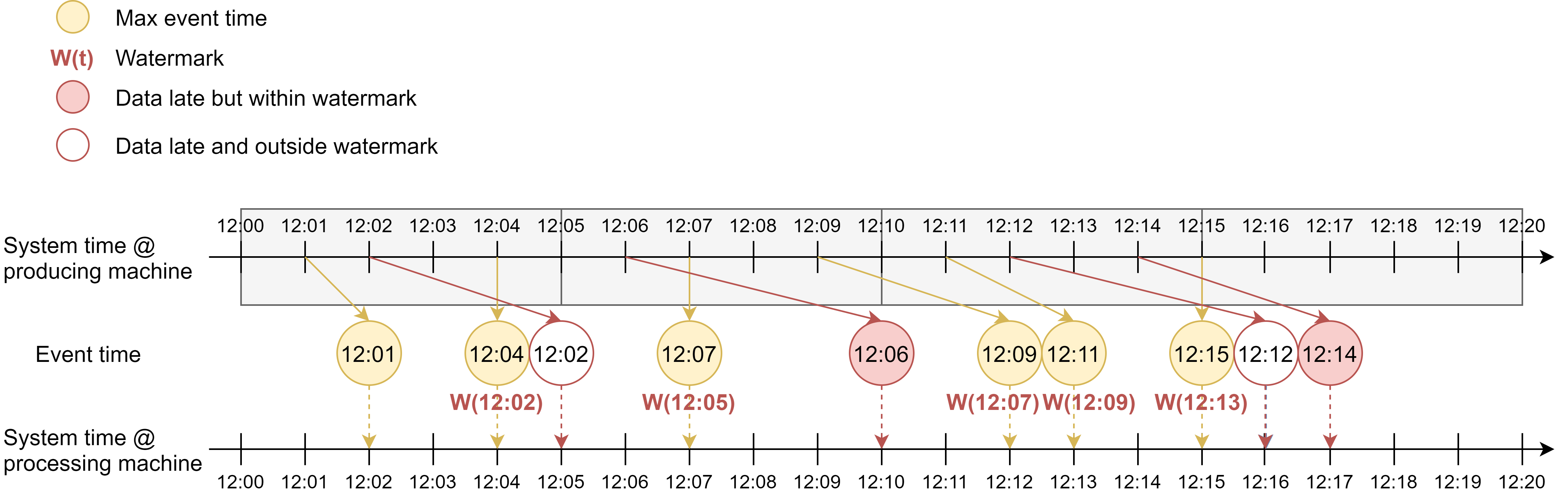
Here is another view of the example. The yellow dotted line connects events that bear the maximum event timestamps observed so far. Each time watermark is updated, it is set to the max event time - 2 min.
We can also adjust the value of the fixed maximum delay. If we want to be more tolerant regarding late events, we can increase the delay to 3 min, and we would have included the event occurred at 12:02 in the watermark line.
If we want to be less tolerant, we can decrease the delay to 1 min, and we would have excluded more late events.
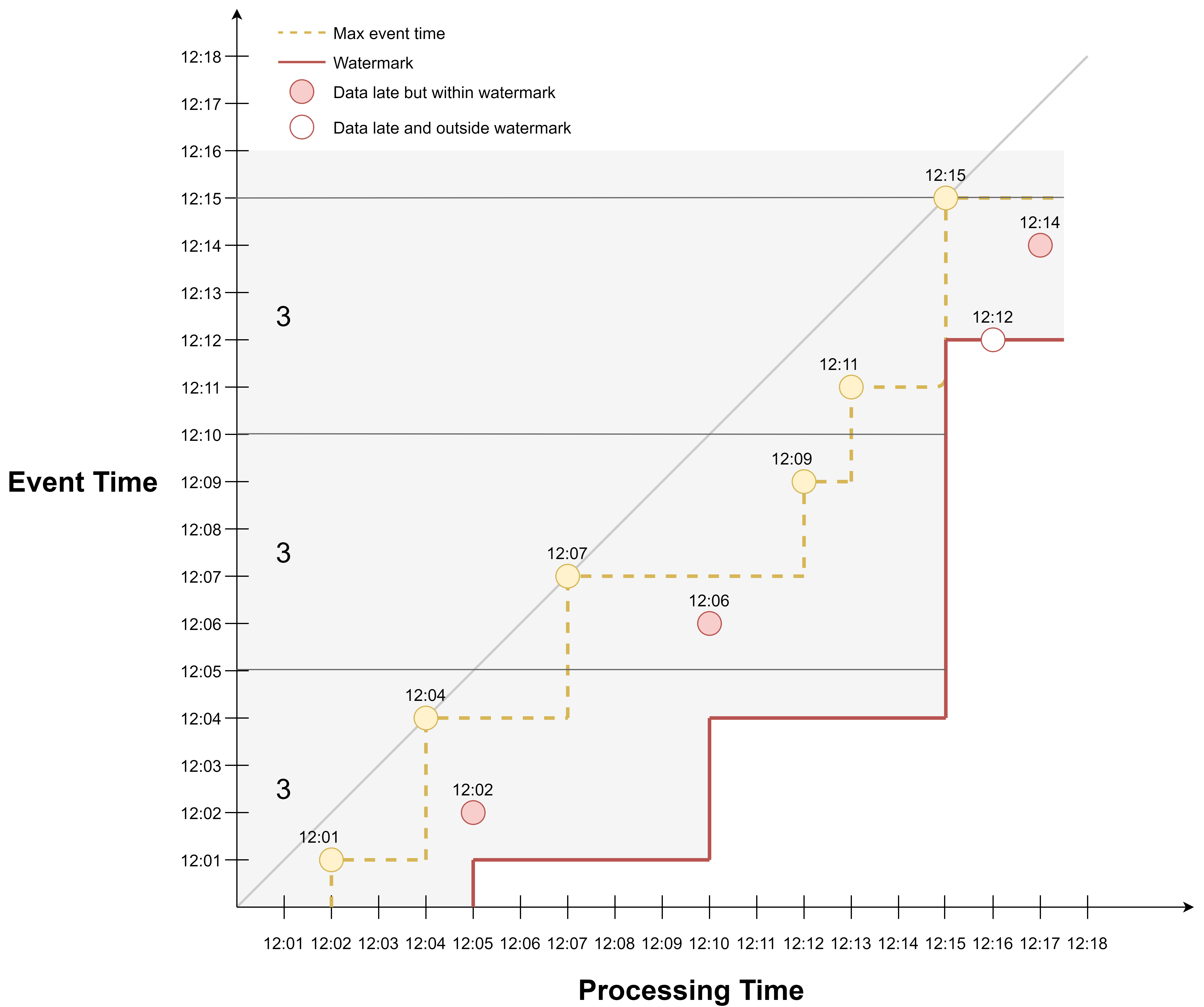
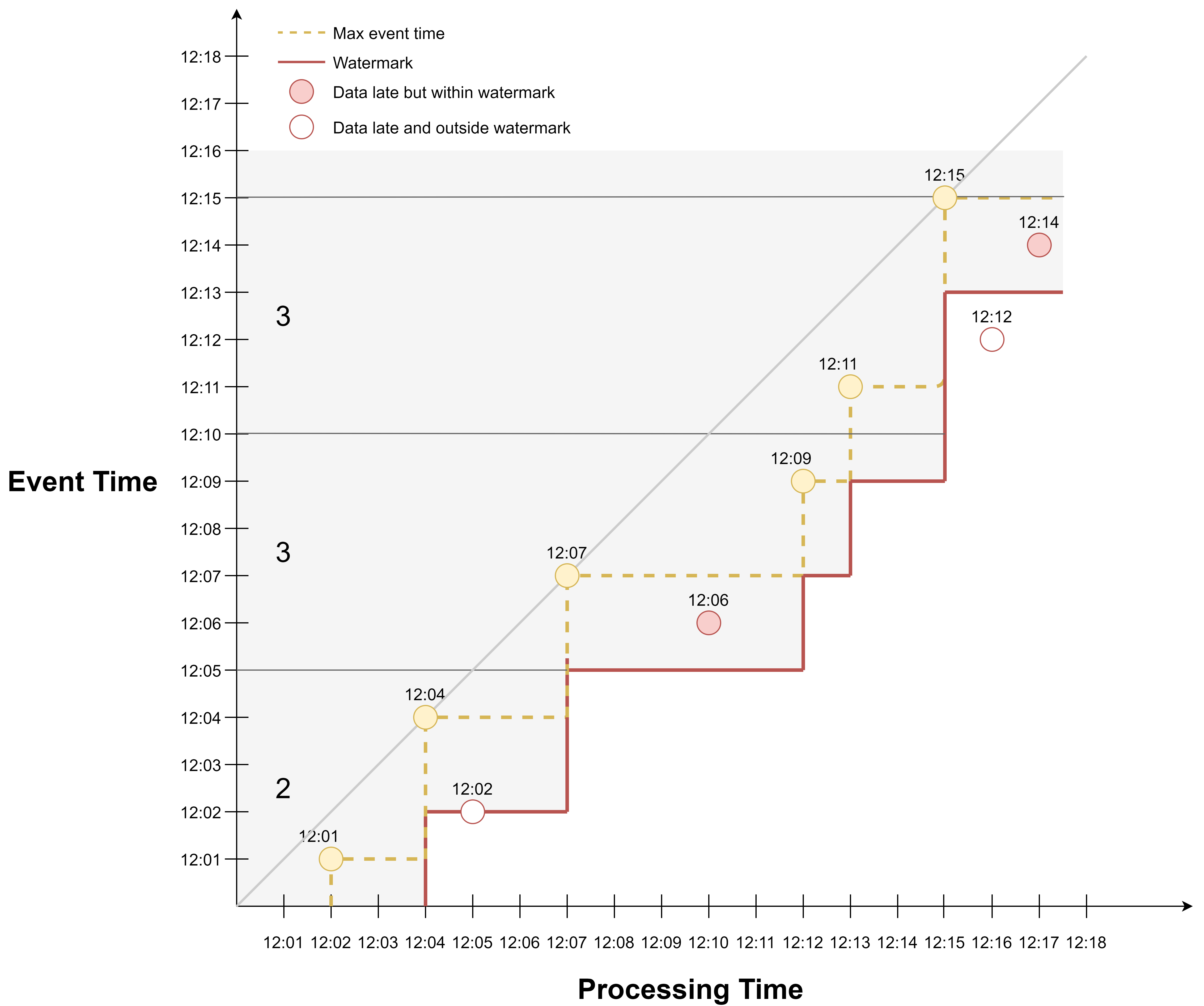
Here is an example of the third watermark generation policy, where watermark is defined as max event time delayed by 2 min, but this time the watermark is generated each time event time advances. It is similar to the last example, just that we have more watermarks because we generate one each time we see a new max event time.
If we apply event time windowing, we would get 2 events in the first window, 3 events in the second window, and 3 events for the third window.
Here is another view of the example.
Because watermark is updated together with max event time, the watermark line is just the max event time line moved downward by 2 min.
Stream Processing Frameworks
That Structured Streaming is based on micro-batch and Flink is based on real streaming underlies many differences in their implementations of window, trigger, watermark, etc.
| Structured Streaming | Flink | |
|---|---|---|
| Model | Batch = Batch Streaming = Micro-batch |
Streaming = Unbounded stream Batch = Bounded stream |
| Operation | Per micro-batch | Per event |
| Time | Processing time Event time |
Processing time Ingestion time Event time |
| Windowing | Tumbling, sliding, session windows | Tumbling, sliding, session windows Custom window |
| Watermark | Fixed delay threshold | Marker that flows within data stream Based on processing time, event time, event, etc |
In general, Flink offers more flexibility when it comes to customizations, which would be helpful for implementing complicated streaming logic.